Random Forest for Regression
In this lesson you will clean datasets using Pandas and Numpy.
Setup
Now that you have learned the basic idea of the random forest model, let's use it to solve a regression problem.
This lesson will also introduce you to Scikit-Learn which is a Python data science module that gives us access to various machine learning algorithms, such as random forest.
The Regression Problem
We want to predict the gas consumption (in millions of gallons) in 48 of the US states based on the petrol tax (in cents), per capita income (dollars), paved highways (in miles) and the proportion of the population with a driving license.
Note: in the dataset we will use, gas is called
petrol.
First, create a new project in Spyder and save it as RandomForestRegression.
Then, create a new file inside the project and save it as regression.py. You can also delete the text that's already in the file.
Create a subfolder in your project called Datasets. Then download the dataset that we will be using and save it into the Datasets folder.
petrol_consumption.csv - A CSV file containing information about petrol consumption.
In your regression.py file, import pandas as pd and numpy as np.
import pandas as pd
import numpy as np
Create a DataFrame using the CSV file 'petrol_consumption.csv'. Remember to create a relative reference to the file using 'Datasets/'
We will also set the Pandas options here so we can see all the columns in our dataset.
import pandas as pd
import numpy as np

pd.options.display.max_columns = None

df = pd.read_csv('Datasets/petrol_consumption.csv')
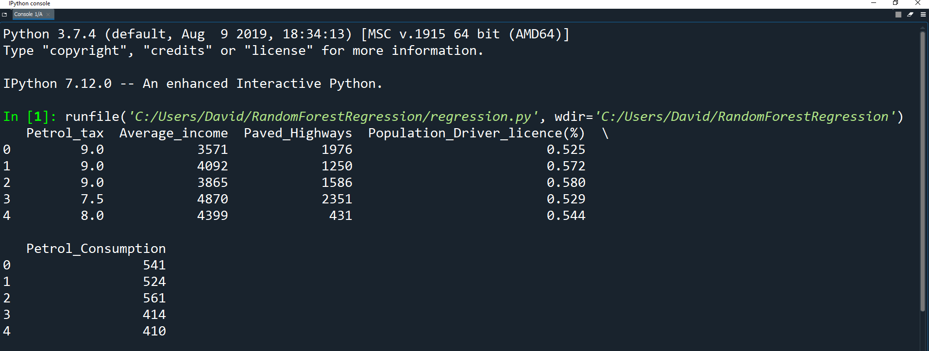
Let's print the first 5 records of the dataset to see what it looks like.
import pandas as pd
import numpy as np

pd.options.display.max_columns = None

df = pd.read_csv('Datasets/petrol_consumption.csv')

print(df.head())
Remember, the first thing we need to do is prepare the data before we can use it. Let's do that now.
Splitting the Data
Before we can teach our model how to predict, we need to divide the data into features and labels sets.
The label (or target) is the value we want to predict, in this case the gas consumption. The features are all the columns the model uses to make a prediction. We will then divide the resulting data into training and test sets.
As you may recall, when we do supervised machine learning, we have to divide the data into two sets:
A training set - used to teach the model how to predict. This set contains input data (the features) that correspond to an output (the labels). The model then predicts results using the input of the training dataset and compares the results to the actual output. Based on the results of the comparison and the algorithm being used, the parameters of the model are adjusted.
A testing set - used to evaluate the performance of the model. Once the model has finished with the training dataset and made its adjustments, it tests itself using the testing set which only contains input data (no output data). We can then use the predictions to check how accurate our model was.
Let's start by dividing the data into features and labels.
As you may recall, we can use iloc[] for position-based indexing. We can index both axes with iloc[] by separating them with a comma. E.g. df.iloc[0, 1] returns the element in row 0, column 1.
There are many different ways to use iloc for indexing which you can learn more about here.
In our case we are going to combine iloc[] with slicing. We can use a colon (:) to select the entire row axis.
We can then specify which columns we want to get using slicing.
df = pd.read_csv('Datasets/petrol_consumption.csv')

X = df.iloc[:, 0:4].values
y = df.iloc[:, 4].values
Here we use slicing to get the first 4 columns for X (indexes 0 to 4 not including 4) and column 5 for y (index 4).
You may notice that we using a capital letter for X (the features) and a lowercase letter for y (the labels). In mathematics, the capital letter (X) represents a matrix of data values and the lowercase letter (y) represents a vector of data values. This is a common naming convention for splitting data in machine learning.
Let's look at what we have data we have in X (our features) and y (our labels).
y = df.iloc[:, 4].values

print("X")
print()
print(X)
print()
print("y")
print()
print(y)
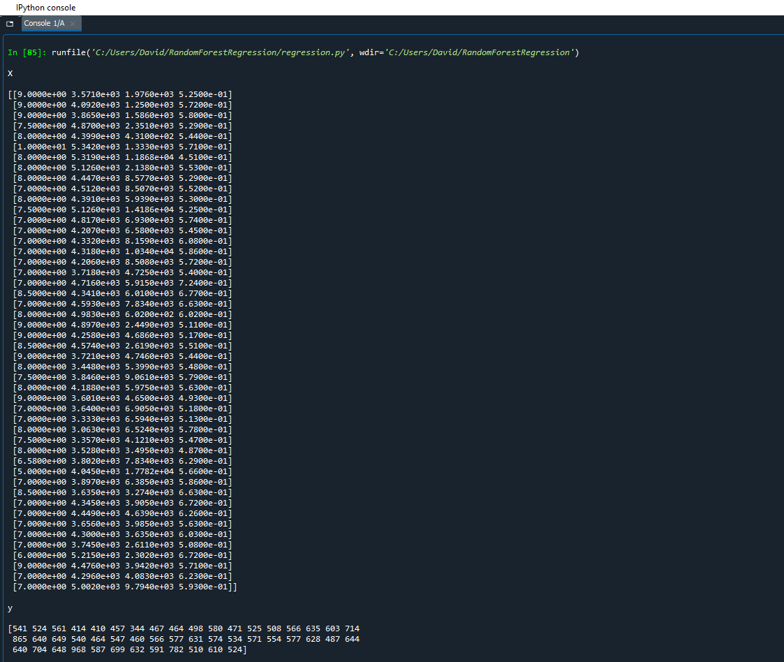
As you can see, X has all the values from our first 4 columns and y has all the values from the final column. The values for X are stored in scientific notation because there is data for 1 column that is a float value. To read scientific notation, 3.5710e+03 just means 3.5710 x (10^ 3) which is equivalent to 3571.
Now we have our features and our labels separated, we can divide the data into training and testing sets using Scikit-Learn. First we have to import train_test_split from sklearn.model_selection.
import pandas as pd
import numpy as np
from sklearn.model_selection import train_test_split
Before discussing train_test_split, you should know about Sklearn (or Scikit-learn).
It is a Python library that offers various features for data processing that can be used for classification, clustering, and model selection.
Model_selection is a method for setting a blueprint to analyze data and then using it to measure new data. Selecting a proper model allows you to generate accurate results when making a prediction.
To do that, you need to train your model by using a training dataset. Then, you test the model against testing dataset.
If you have one dataset, you'll need to split it by using the Sklearn train_test_split function first.
Now we can use the train_test_split() method to split up our data.
X = df.iloc[:, 0:4].values
y = df.iloc[:, 4].values

X_train, X_test, y_train, y_test = train_test_split(X, y, test_size=0.2, random_state=0)
This is a long line of code, so let's take a moment to understand each part:
train_test_split() is a function in Sklearn model selection for splitting data arrays into two subsets:
one for training data and another for testing data. With this function, you don't need to divide the dataset manually.
By default, Sklearn's train_test_split() will randomly divide the dataset into two. However, you can also specify a random state for the operation.
There are a few parameters in train_test_split that we need to look at:
Output:
X_train - variable to hold the training dataset
X_test - variable to hold the test dataset
y_train - variable to hold the set of labels that correspond to the data in X_train
y_test - variable to hold the set of labels that correspond to the data in X_test
Parameters:
X, y - the first parameter is the dataset you're selecting to use.
test_size - a percent (represented as a float value from 0 to 1) that sets the size of the testing dataset. It will be set to 0.25 if the training size is not specified.
random_state - if you do not pass a value into this parameter, it will perform a different random grouping of the training and testing splits every time. If you pass in a number, it will perform the split consistently every time the function is called.
By default, Sklearn's train_test_split() will randomly divide the dataset into two. However, you can also specify a random state for the operation.
There are a few parameters in train_test_split that we need to look at:
X_train, X_test, y_train, y_test = train_test_split(X, y, test_size=0.*, random_state=*)
Output:
X_train - variable to hold the training dataset
X_test - variable to hold the test dataset
y_train - variable to hold the set of labels that correspond to the data in X_train
y_test - variable to hold the set of labels that correspond to the data in X_test
Parameters:
X, y - the first parameter is the dataset you're selecting to use.
test_size - a percent (represented as a float value from 0 to 1) that sets the size of the testing dataset. It will be set to 0.25 if the training size is not specified.
random_state - if you do not pass a value into this parameter, it will perform a different random grouping of the training and testing splits every time. If you pass in a number, it will perform the split consistently every time the function is called.
  X = df.iloc[:, 0:4].values
  y = df.iloc[:, 4].values

  X_train, X_test, y_train, y_test = train_test_split(X, y, test_size=0.2, random_state=0)
So as you can see from our usage, we split the data so that 20% of the data is randomly selected to go into the test set.
This leaves 80% of the data to be randomly placed into the training set. The 80-20 ratio is fairly standard for train-test splitting, but once you perform you finishing setting up the code for this assignment, feel free to change the split amounts and see how that alters the accuracy of the machine learning algorithm.
Feature Scaling
When we look at the dataset, you can see that the values aren't scaled very well. For example, the Petrol_tax column has values in the range of tens, while the Average_Income column has values in the thousands. We can fix this using feature scaling.
Feature scaling is a method used to normalize the range of independent variables (features) of data.
It is also known as data normalization.
Most of the time, your dataset will contain features highly varying in magnitudes, units, and range. Since most machine learning algorithms use Euclidean distance between two data points in their computations, this is a problem.
The algorithms only take in the magnitude of features and ignore the units. Therefore results would vary greatly between different units, such as 5 kilograms and 5000 grams, even though they are the same The features with high magnitudes will matter much more in the machine learning algorithm's distance calculations than features with low magnitudes.
Therefore we use feature scaling to normalize our data into a fixed range.
We can scale our data using Scikit-Learn's StandardScaler class from sklearn.preprocessing. First, let's go back to the top of our file and import it.
import pandas as pd
import numpy as np
from sklearn.model_selection import train_test_split
from sklearn.preprocessing import StandardScaler
Now we can create a StandardScaler object and use its methods to scale our data.
We only need to scale our X_train and X_test because these are our features. We do not need to scale our labels (y_train and y_test).
X_train, X_test, y_train, y_test = train_test_split(X, y, test_size=0.2, random_state=0)

sc =  StandardScaler()
X_train = sc.fit_transform(X_train)
X_test = sc.transform(X_test)
First we created a StandardScaler object and assigned it to sc.
Then we used the sc.fit_transform() method on X_train to scale the data.
Finally we used the sc.transform() method on X_test to perform standardization by centering and scaling the data.
There is some underlying math happening here so don't worry if you don't fully understand it. Just know that these two methods are used to automatically normalize the data in the training set and the testing set, and that once you use fit_transform() on one data set, you use transform() on other data sets of the same shape.
You can learn more about the StandardScaler here.
Training the Algorithm
Finally, we can train our random forest algorithm and solve the regression problem.
First we must create a RandomForestRegressor which is used in regression problems using random forest. Because someone has already implemented the complicated math behind the machine learning algorithm, all we need to do is import the class that runs the machine learning algorithm and use it.
As always, we must import this class at the top of our file. This class comes from the sklearn.ensemble library.
import pandas as pd
import numpy as np
from sklearn.model_selection import train_test_split
from sklearn.preprocessing import StandardScaler
from sklearn.ensemble import RandomForestRegressor
Now we can create the RandomForestRegressor object.
sc =  StandardScaler()
X_train = sc.fit_transform(X_train)
X_test = sc.transform(X_test)

regressor = RandomForestRegressor(n_estimators=20, random_state=0)
Here the n_estimators parameter is used to define the number of trees in the random forest. We will start with 20 and see how the model performs.
We set the random_state parameter to 0 to make the algorithm deterministic. This way, every time we run the algorithm, the output will always be the same.
There are other parameters you could use which you can learn more about here.
Now we can can actually run the algorithm on our dataset using the regressor.
regressor = RandomForestRegressor(n_estimators=20, random_state=0)

regressor.fit(X_train, y_train)
y_pred = regressor.predict(X_test)
regressor.fit() takes in our training set as arguments and builds a forest of trees. Fit is just Scikit-Learn's name for training the model.
regressor.predict() then makes predictions based on our testing test, and we store the predictions in y_pred.
Evaluating the Algorithm
Now that we have trained the algorithm against our data sets and gotten back predictions using the testing set, we should check how well our model performed.
For regression problems, there are 3 metrics used to calculate how erroneous (wrong) an algorithm is based on the predicted value and the actual value.
These metrics used to evaluate an algorithm are:
Mean Absolute Error: this is the average of all the differences between your predicted values and the actual values. For example, if you predicted 60 and the actual value was 63.5, you would have an absolute error of 3.5. - Learn more about mean absolute error.
Mean Squared Error: This is the average of all the errors squared. By squaring the numbers, you assign greater weight to differences that are larger. For example, if you predicted 63 but the actual value was 60, you would have a squared error of 9. If you predicted 65 but the actual value was 60, you would have a squared error of 25. If you have a low mean absolute error but a high mean squared error, it means that there are outliers in the data set where the errors were unusually large, even though most of the predictions were accurate. - Learn more about mean squared error.
Root Mean Squared Error: When you square each of the errors, it results in a number that is very large compared to the mean absolute error. By taking the square root, it will result in a number that is more easily directly comparable to the mean absolute error. - Learn more about root mean squared error.
Let's import the metrics class in order to calculate these values.
import pandas as pd
import numpy as np
from sklearn.model_selection import train_test_split
from sklearn.preprocessing import StandardScaler
from sklearn.ensemble import RandomForestRegressor
from sklearn import metrics
Now we can calculate the metrics using our testing values (y_test) and the predicted values (y_pred).
regressor.fit(X_train, y_train)
y_pred = regressor.predict(X_test)
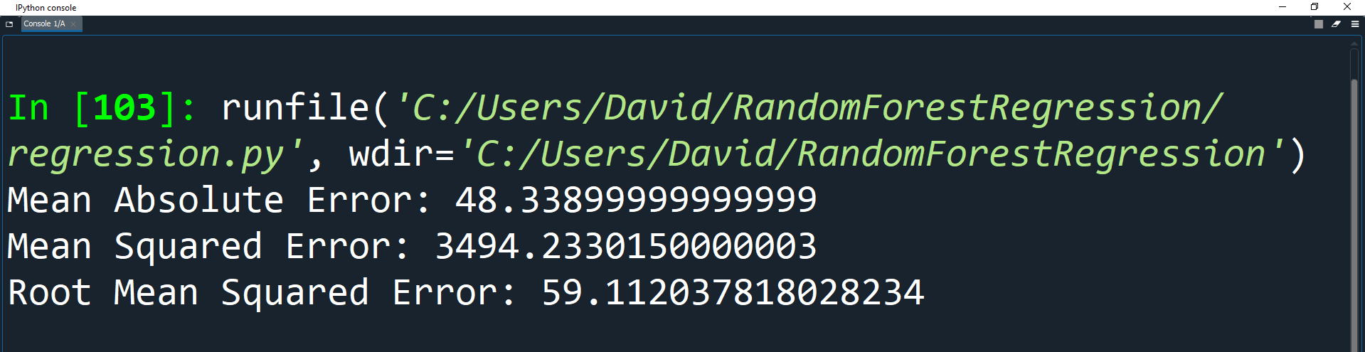
print('Mean Absolute Error:', metrics.mean_absolute_error(y_test, y_pred))
print('Mean Squared Error:', metrics.mean_squared_error(y_test, y_pred))
print('Root Mean Squared Error:', np.sqrt(metrics.mean_squared_error(y_test, y_pred)))
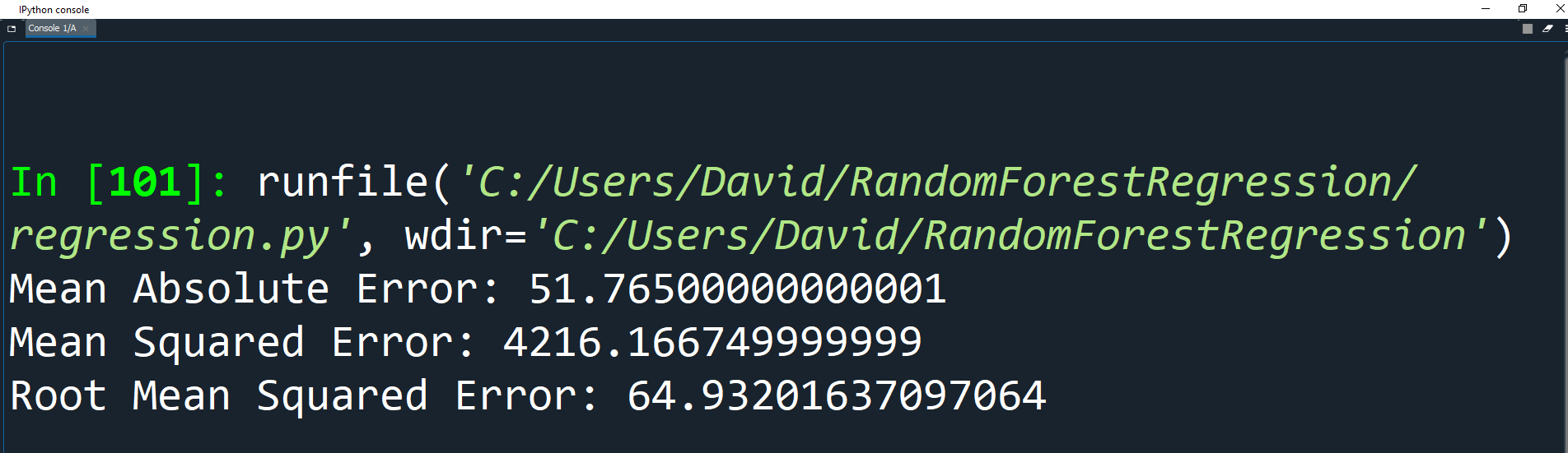
The average consumption of gasoline is 576.77. But with only 20 trees, the root mean squared error is 64.93 which is greater than 10% of the average consumption.
This could be for many reasons, but may mean that we did not use enough estimators (trees).
Let's change the number of estimators to 200, run the program again, and see what happens.
regressor = RandomForestRegressor(n_estimators=200, random_state=0)

regressor.fit(X_train, y_train)
y_pred = regressor.predict(X_test)
Great! The metrics show that increasing the estimators has in fact decreased the errors in our algorithm. You can change the number of estimators to be even higher, but that will cause the algorithm to run slower. Ultimately, you want to find the minimum number of estimators that gives you the best result for the algorithm based on the data set you have, so that your model is both fast to train and accurate in its results.
You can also change the random state integer, and see if a different combination of the training and test data set will yield more accurate results. However, use this technique sparingly. If you spend too much time trying to find the perfectly split dataset, you might overfit the data, which means it will work well for your dataset, but not for other data inputs you have the model predict results for.
Activity: Analyze Datasets
- Would this dataset be a good candidate to use a supervised learning algorithm?
- Could there be links between features that could be used to make predictions?
- What type of cleanup would be needed to make the dataset ready for machine learning?
Now that you know how to use the random forest algorithm, take another look at the datasets that you found and cleaned in earlier lessons.
Based on what you know about the random forest algorithm and supervised learning algorithms:
If you find a dataset that you think could be used to make a prediction, try it out!