Handwritten Digit Recognition
This lesson will teach you how to create a program that recognizes handwritten digits.
Setup
We're going to continue the use of support vector machines to solve another classification problem. This time we are going to classify handwritten digits so we will be able to feed in a picture of a digit and the program should tell us what it is.
First create a new project in Spyder and save it as DigitRecognition.
Then, create a new file inside the project and save it as recognition.py. You can also delete the text that's already in the file.
In your recognition.py file, we are going import all of our necessary modules and classes:
Modules for Analysis:
pandas - for datasets
numpy - for arrays
svm from sklearn - for the svm algorithm (we will also set the font for our visuals to be slightly bigger using sns.set(font_scale = 1.2))
metrics from sklearn - module for evaluating the performance of the model
Modules for Visuals:
matplotlib.pyplot - for graphs
seaborn - prettier graphs (we will also set the font for our visuals to be slightly bigger using sns.set(font_scale = 1.2))
New Module:
We will also import tensorflow here as tf.
Tensorflow is another machine learning library with many uses. For now we are just using it to get the mnist dataset.
The mnist dataset is a large set of images of handwritten digits. There are 60,000 training images and 10,000 testing images!
import pandas as pd
import numpy as np
from sklearn import svm
from sklearn import metrics
import matplotlib.pyplot as plt
import seaborn as sns; sns.set(font_scale=1.2)
import tensorflow as tf
There are many ways to get the mnist dataset, but we are going to get it from TensorFlow's Keras. Keras is a neural network library that we can run with TensorFlow. It also contains many datasets such as the mnist dataset that we will use.
Luckily, using this dataset has two major advantages:
The dataset is already clean and ready for use.
We can load the dataset straight into the training set and testing set, each with the features and labels separated.
Creating an image classification machine learning algorithm can be a lot of work from the amount of data required to generate accurate results.
We will use the function load_data() function from Keras which returns two tuples.
import pandas as pd
import numpy as np
from sklearn import svm
from sklearn import metrics
import matplotlib.pyplot as plt
import seaborn as sns; sns.set(font_scale=1.2)
import tensorflow as tf

(X_train, y_train), (X_test, y_test) = tf.keras.datasets.mnist.load_data()
The first tuple contains the training set features (X_train) and the training set labels (y_train). The second tuple contains the testing set features (X_test) and the testing set labels (y_test).
This is similar to how train_test_split() returned its arrays for testing and training.
X_train and X_test are our array of images while y_train and y_test are our array of labels for each image.
For example, if the image shows a handwritten 7, then the label will be the integer 7.
After running this code the first time, you might see some initial messages in the console displaying the steps that the code is taking to download the dataset. You may see some warning messages, but as long as there are no error messages the dataset will be downloaded and we can use it for our image recognition project.
Displaying the Images
Now we have our images imported and divided into their groups. Let's display one of the images to see what it looks like.
We can easily do this using matplotlib's imshow() function which simply displays an image.
(X_train, y_train), (X_test, y_test) = tf.keras.datasets.mnist.load_data()

plt.imshow(X_train[0], cmap='gray')
plt.show()
Here we pass X_train[0] into the imshow() function so it will display the first element (image) from the X_train set.
We also set the cmap parameter to 'gray' to indicate the images do not contain color information.
As always, we call the show() function to actually show the image on the screen.
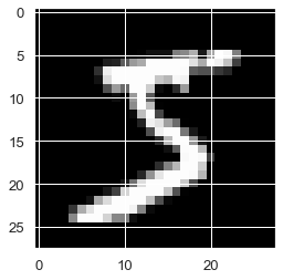
Look in the plots tab and you should see the first number displayed as a plot. A handwritten number 5!
You will notice that the image appears black and white and that each axis of the plot ranges from 0 to 28. This is because of the format that all the images in the dataset have:
1. All the images are grayscale, meaning they only contain black, white and gray.
2. The images are 28 pixels by 28 pixels in size (28x28).
Let's print one of the elements (images) from X_train to the console to see what the actual data of the image is like.
(X_train, y_train), (X_test, y_test) = tf.keras.datasets.mnist.load_data()

print(X_train[0])
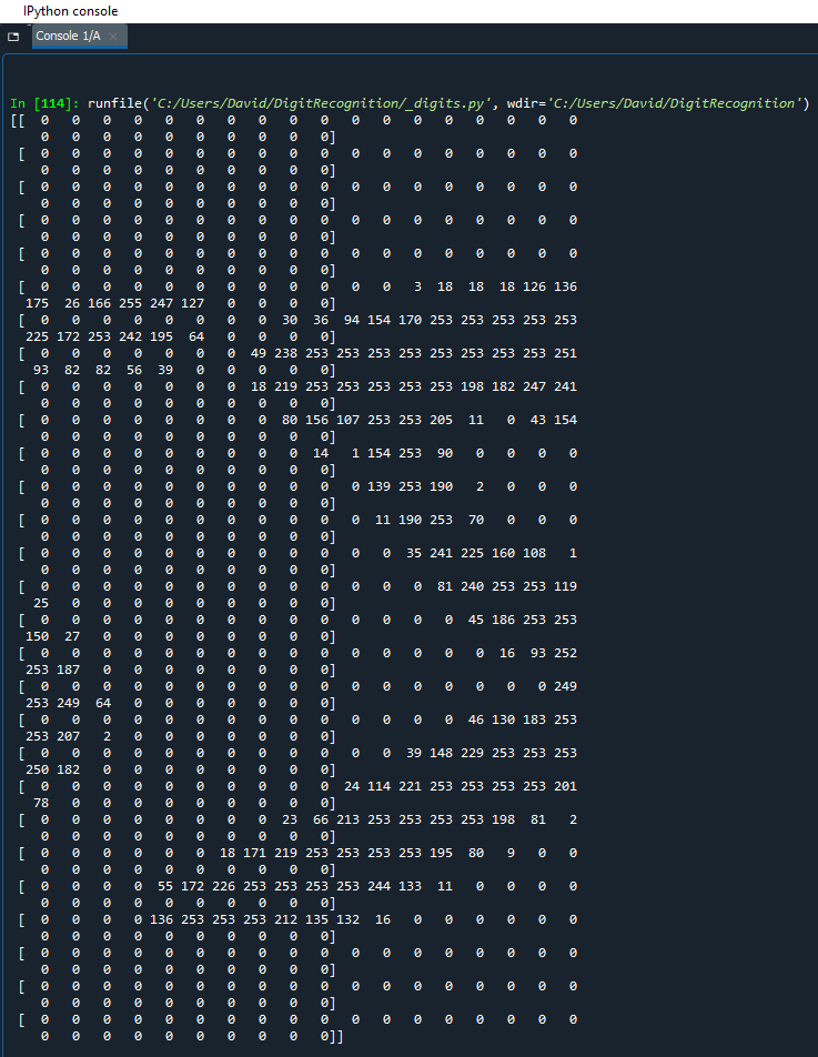
As you can see in the console, the image data is just an array of digits. You can almost make out a 5 from the pattern of the digits in the array.
If you look closely at the data, you will see that it is actually a 2D array [28][28]. It is an array of 28 arrays, each with 28 values inside them. Each value is just one pixel, hence why we get 28x28 pixels (784 pixels in total).
Okay, so we have an array of values that represent pixels, but how does one number equal a black, white or gray pixel on an image?
In computers, a grayscale pixel is stored as a digit between 0 and 255 where 0 is black, 255 is white and values in between are different shades of gray.
Therefore, each value in the [28][28] array tells the computer which color to put in that position when we display the actual image.
Remember the cmap parameter we used in the imshow() function? Well, cmap is actually short for color map and is used to map scalar data (numbers) to colors.
In this case, because our images are grayscale, we can set cmap to
grayso that it maps the digits in the array to a color on the grayscale: black, white or a shade of gray.
Fixing the Data
Although the dataset is clean, we still have to do some data treatment like any good data scientist.
Specifically, we have to reformat our X_train array and our X_test array because they do not have the correct shape.
Let's print the shape of all our arrays just to see what they currently look like. We will use the shape attribute to do this.
(X_train, y_train), (X_test, y_test) = tf.keras.datasets.mnist.load_data()

print("X_train shape", X_train.shape)
print("y_train shape", y_train.shape)
print("X_test shape", X_test.shape)
print("y_test shape", y_test.shape)
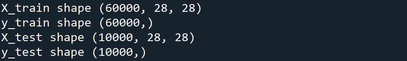
Here you can see that for the training sets we have 60,000 elements and the testing sets have 10,000 elements.
y_train and y_test only have 1 dimensional shapes because they are just the labels of each element.
X_train and X_test have 3 dimensional shapes because they have a width and height (28x28 pixels) for each element.
Whenever we fit our model, we need to pass two arguments into the fit() function:
X: Training data of shape (n_samples, n_features)
y: Training label values of shape (n_samples, n_labels)
Whenever we predict with our model, we need to pass one argument into the predict() function:
X: Testing samples of shape (n_samples, n_features)
Basically, supervised learning algorithms in scikit-learn expect data to be stored in two-dimensional arrays.
Luckily, 1D arrays such as our labels in y_train and y_test, are automatically reshaped to become 2D arrays. Therefore they will be reshaped from (n_samples,) to (n_samples, 1)
However, our features are still in 3 dimensions with a shape (n_samples, 28, 28). We need to reshape this to be only 2 dimensional.
We will do this by changing the pixel data to not be a 2D array of height and width, but one long array of all the pixels. I.e. 28 pixels by 28 pixels will just become 784 pixels (28 squared).
Let's reshape X_train and X_test. Remember that X_train has 60,000 elements, each with 784 total pixels so it will become shape (60000, 784).
Whereas X_test has 10,000 elements, each with each with 784 total pixels so it will become shape (10000, 784).
(X_train, y_train), (X_test, y_test) = tf.keras.datasets.mnist.load_data()

X_train = X_train.reshape(60000, 784)
X_test = X_test.reshape(10000, 784)
Fitting the SVM Model
Now that our arrays are in good shape, we can actually create our model and start training. However, there's one last thing we're going to do before we start training.
Currently we have 60,000 records for training and 10,000 records for testing. This is a huge amount of data and will take a large amount of time to process. It could take hours, days, even weeks.
To avoid this, we are just going to use a portion of the dataset. So let's take the first 100 elements and use those instead.
X_train = X_train.reshape(60000, 784)
X_test = X_test.reshape(10000, 784)

X_train = X_train[:100, :]
y_train = y_train[:100]
X_test = X_test[:100, :]
y_test = y_test[:100]
Here we use slicing to get the first 100 rows of images and labels for both the training and testing sets. We also make sure to keep all the columns for the X sets (our features) since we still need all 784 pixels.
Finally we can create our machine learning model and train it!
Create the support vector classification model using svm.SVC(). Then fit the model with the X_train set and the y_train set.
X_train = X_train[:100, :]
y_train = y_train[:100]
X_test = X_test[:100, :]
y_test = y_test[:100]

model = svm.SVC()
model.fit(X_train, y_train)
Our model is now trained and ready to be tested on a fresh set of data. Let's use our testing set of images so our model can predict their labels.
model = svm.SVC()
model.fit(X_train, y_train)

y_pred = model.predict(X_test)
Let's also write some code so that we can display any image we want from the dataset. This will allow us to compare the predictions to the actual images.
y_pred = model.predict(X_test)

index_to_compare = 0

title = 'True: ' + str(y_test[index_to_compare]) + ', Prediction: ' + str(y_pred[index_to_compare])

plt.title(title)
plt.imshow(X_test[index_to_compare].reshape(28,28), cmap='gray')
plt.grid(None)
plt.axis('off')
plt.show()
Here we create a variable for the index of the image that we want to compare to its prediction. We'll try the first image which is at index 0.
Then we display our image in a nice format:
We create a title which displays both the true label of the image and our model's predicted label.
We pass the image into imshow() and set the cmap to
gray. Here we also have to reshape the image data which is currently (784,), back to (28,28).
Finally, we turn off the grid and axis since we're not displaying a graph, and we show the image to the screen.
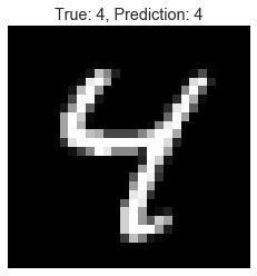
Here is what you will see for index 0.
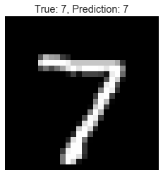
In the Plots tab you will see the image is of a handwritten number 7, which the true label confirms.
Therefore our model was correct in predicting that it was a 7. Fantastic!
You can change the value of index_to_compare to see other images and their respective predictions. For example, let's look at the third image in the test set (index 2).
index_to_compare = 2
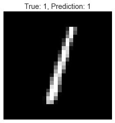
This time the image is of the digit 1, and our model predicted a 1.
Now let's look at the seventh image in the set (index 6).
index_to_compare = 6

Oh no! Our model's prediction was wrong this time. It predicted a 9 but the image was actually of the digit 4. Clearly our model isn't as good as we thought.
Evaluating the Model
Let's try and figure out why our model is not doing too well.
We can look at the accuracy of the model using the metrics.accuracy_score() function.
plt.show()

acc = metrics.accuracy_score(y_test, y_pred)
print('\nAccuracy: ', acc)

As you can see, the accuracy of our model is only 0.68 (68% accurate). This means that over 30% of the model's predictions are wrong. This model definitely has room for improvement.
Why is it so inaccurate?
There are many factors that affect the accuracy and performance of a machine learning model.
In this case, there is one major factor that is affecting the accuracy: the sample size.
Since we reduced our sample size to 100, this is not many images for the model to train on.
It also means that with only 100 images, there will only be an average of 10 images for each handwritten digit.
However, that's just an average. There may be only 1 image for one type of digit and 19 for another type of digit.
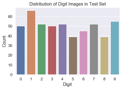
Let's use Seaborn to create a pretty graph that visualizes the actual distribution of images for each digit in our sample.
acc = metrics.accuracy_score(y_test, y_pred)
print('\nAccuracy: ', acc)

digits = pd.DataFrame.from_dict(y_train)

ax = sns.countplot(x=0, data=digits)

ax.set_title("Distribution of Digit Images in Test Set")
ax.set(xlabel='Digit')
ax.set(ylabel='Count')

plt.show()
Here we create a DataFrame using the array of labels from the training set (y_train) so we can pass it into our plot function.
Then we use Seaborn's countplot() function to create an axes object with the plot on it. We set the x parameter to 0 which will label the x-axis and we set the data parameter to our digits DataFrame.
Finally we set the title and change the labels for the x and y axis. Then we show the plot.
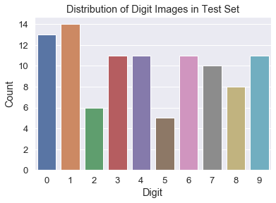
As you can see, with only 100 samples, the images for each digit are not distributed very evenly. For example, there are many images of digit 1 but very few images of digit 5.
A common way to visualize the accuracy of a classification model is with a confusion matrix and a heatmap.
A confusion matrix (also known as an error matrix) is a table that compares predicted classifications to actual classifications.
A heatmap uses intensity of the intensity of colors to represent the amount of a category.
First, we will create the confusion matrix. This can be done easily with the metrics.confusion_matrix() function.
plt.show()

cm = metrics.confusion_matrix(y_test, y_pred)
print(cm)
Here we create the confusion matrix by passing our test labels and our predicted labels into the metrics function.
Then we print the matrix to the console.
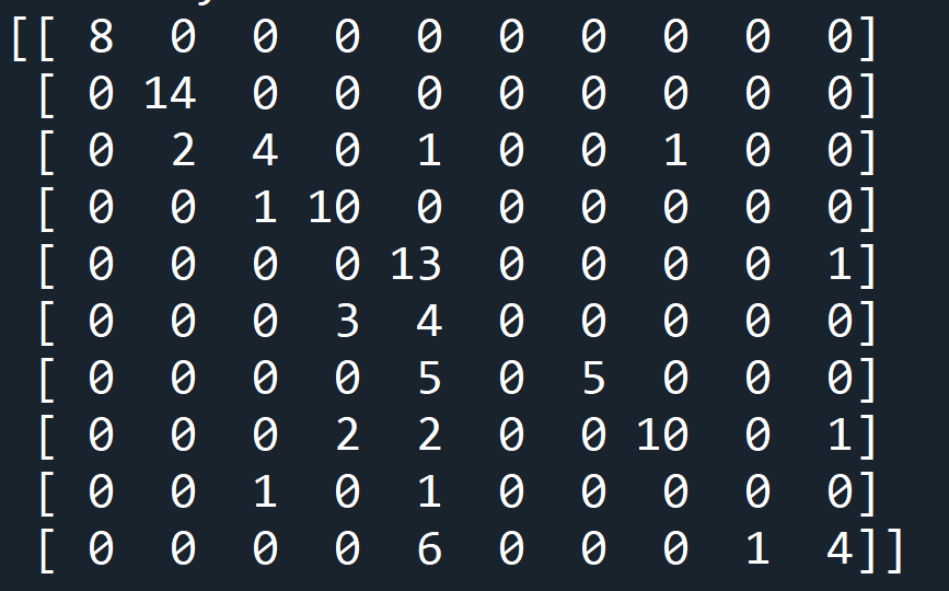
Look at the matrix as a graph where the x axis is the predicted labels from 0 to 9 and the y axis is the true labels from 0 to 9.
The numbers at each point represents the number of matches made between a prediction and a true label.
The diagonal line of numbers from the top-left to the bottom-right of the grid shows perfect matches where the prediction for the label was correct. The outliers are where the model made false predictions.
Now, let's create a heatmap as another way to visualize this data.
cm = metrics.confusion_matrix(y_test, y_pred)
ax = plt.subplots(figsize=(9, 6))
sns.heatmap(cm, annot=True)
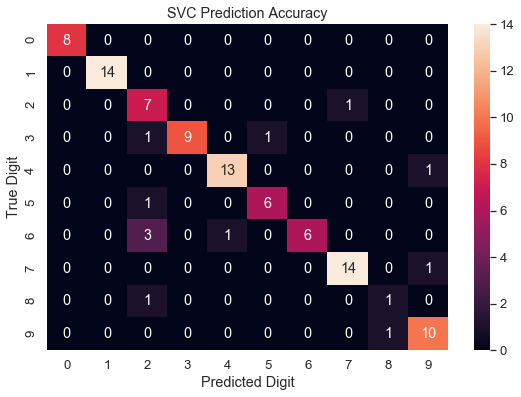
ax[1].title.set_text("SVC Prediction Accuracy")
ax[1].set_xlabel("Predicted Digit")
ax[1].set_ylabel("True Digit")
plt.show()
We first created a plot with a size of 9 inches by 6 inches using the subplots() function which returned an Axes object.
We then create a Seaborn heatmap by passing in our confusion matrix (cm). We also set the annot parameter to True which means the heatmap will have annotations for the number of matches at each point.
We then add a title and change the label for the x-axis and the y-axis. Finally we show the plot.
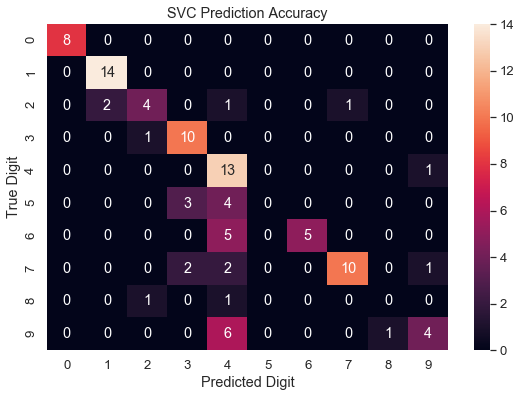
Beautiful! You can now clearly see where the predictions were correct and where they were wrong for each digit.
Now we can see that quite a lot of predictions were wrong, especially looking at how many times the model wrongly predicted 4.
We want to get it so that our heatmap shows a clear diagonal line with minimal deviation. Therefore, we should now try to improve our model so we have a better accuracy, sample distribution, and heatmap.
Let's go back and raise the number of training samples we use to fit the model. This time we will use 500 samples.
X_train = X_train[:500, :]
y_train = y_train[:500]
X_test = X_test[:100, :]
y_test = y_test[:100]

model = svm.SVC()
model.fit(X_train, y_train)
Let's run the program again and see if our model has improved. We will start by looking at the distribution graph.
Great! The distribution of images for each digit looks a lot more even now. How about the accuracy?

Amazing! The accuracy has increased from 0.68 all the way to 0.88. That's a substantial increase in the accuracy of the model. Finally, how does our heatmap look?
Fantastic! The diagonal line shows a much better accuracy of predictions now with many fewer false predictions.
If you still have the index_to_compare variable set to 6, this should also have been displayed.
If you remember from before, our model falsely predicted this image to be a 9. Now it is correctly predicting it to be 4.
Now you understand that the sample size used to train a model can hugely affect how well it performs.
You just have to find the right balance between using enough data to make the model accurate while not using so much data that the model takes too long to train.
Try training the model with different amounts of data from the training set and see what works best for you. For now, we have a much better model that we can use to predict handwritten digits.
Activity: Image Recognition
Now that you have the tools to put together an image recognition algorithm, you can find image-based data sources and attempt to perform classification tasks on those images.