NumPy
This lesson will teach you how to use NumPy (or numpy) which is a third-party package for numerical computing in Python.
What is NumPy?
NumPy is one of the most important python packages for scientific computing.
NumPy brings arrays to python, which are similar to lists but are more useful for data science and machine learning.
NumPy also allows for many fast mathematical processes and we will look at 3 in particular:
Multidimensional Arrays: Arrays with more than 1 dimension
Broadcasting: Applying changes to all elements in an array
Indexing: Finding data at specific array locations
If you have issues with using numpy on your computer, then reference the Python Setup Guide on how to install packages to your computer using Pip.
NumPy Arrays
Create a new python file and save it as usingNumpy.py.
Like Lists, numpy arrays store collections of data. However numpy arrays are faster and give you the ability to perform calculations across entire arrays very quickly.
To use numpy, we must first import it. We can do this by writing import numpy.
import numpy as np
This line imports numpy and abbreviates it to np using the as keyword (this is called aliasing modules). This is common practice for packages that have long names.
We must create a numpy array from a list. We can do this in two ways:
Assign a list to a variable then pass the variable into the parentheses of numpy.array()
Create the list directly in the parentheses of numpy.array()
import numpy as np

# Method 1
numbers = [2,4,6,8,10]
np_numbers_1 = np.array(numbers)

# Method 2
np_numbers_2 = np.array([2,4,6,8,10])
Using numpy arrays we can perform element-wise calculations. This is when we apply a calculation to each object in the array.
These operations are very fast and efficient which is important for data science as you may have 1000's of items in an array which will take longer to compute.
import numpy as np

height = [2.5, 5.7, 12.3, 4.1, 8.7]
width = [15.3, 13.6, 8.1, 6.5, 7.4]

np_height = np.array(height)
np_width = np.array(width)

area = np_height * np_width

print(area)

# Output:
# [38.25 77.52 99.63 26.65 64.38]
This code takes all 5 height and width values and calculates the area for each one.
It works by going through both arrays and multiplying the values with the same index. For example,
2.5is multiplied with
15.3.
We can also get specific elements of a numpy array based on a condition. This is called boolean array indexing. This concept might sound familiar. Boolean array indexing uses the same principles as filtering on a list with a lambda function. But in this circumstance, the filter is written a little bit differently.
You start by writing the name of the array along with square brackets. In this case, the newly created array we're using is area.
area[]
Then, the inside of the square brackets should have the
resultthat you would have specified inside the lambda function. In this case, this boolean array index will return all results inside the array that are less than 50 and store it inside the small_areas variable.
area[area < 50]
import numpy as np

height = [2.5, 5.7, 12.3, 4.1, 8.7]
width = [15.3, 13.6, 8.1, 6.5, 7.4]

np_height = np.array(height)
np_width = np.array(width)

area = np_height * np_width

small_areas = area[area < 50]

print(small_areas)

# Output:
# [38.25 26.65]
This is a circumstance where the concept of filtering is present, but the syntax for the filter is different to make the process easier for data scientists using this package. Because numpy arrays use the concept of filtering so much, its syntax is designed to be very easy to use.
Multidimensional Arrays
Think of a numpy array as a grid of values.
The ones we have looked at so far are called 1-D (one-dimensional) arrays because they have just 1 row of values.
However, we can create arrays that look more like grids with rows and columns. These are multidimensional arrays.
import numpy as np

a = np.array([1,2,3]) # 1-D array

b = np.array([[1,2,3],[4,5,6]]) # 2-D array
As shown in the example above, the 2-D (two-dimensional) array is made of an array where each element is also an array.
The number of dimensions is the rank of the array. So the 1-D array has rank 1 and the 2-D array has rank 2.
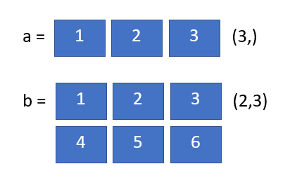
The shape of an array is a tuple of integers showing the size of the array along each dimension. We can see the shape of an array by looking at the .shape property of the array.
import numpy as np

one_d_array = np.array([1,2,3]) # 1-D array

two_d_array = np.array([[1,2,3],[4,5,6]]) # 2-D array

print(one_d_array.shape) # Prints '(3,)'

print(two_d_array.shape) # Prints '(2, 3)'
The first array shows a shape of
(3,)because it has 3 elements in 1 dimension.
The second array shows a shape of
(2,3)because the outer dimension has 2 elements, and the inner dimensions have 3 elements.
You can make arrays with even more dimensions, but in machine learning we most commonly use 2-D arrays.
Broadcasting
Like we saw before, the simplest case for performing math on arrays is when they are both the same shape.
In the example below, both arrays have a shape of (3,) meaning they are 1-D arrays with 3 elements each.
import numpy as np

np_numbers1 = np.array([1,2,3])
np_numbers2 = np.array([4,5,6])

sum = np_numbers1 + np_numbers2

print(sum)

# Output:
# [5 7 9]
Broadcasting gives us the ability to work with arrays of different shapes using arithmetic operations.
A lot of the time we will have a smaller array and a larger array and we will need to use the smaller array multiple times to perform some operation on the larger array.
The simplest broadcasting case is when an array and a scalar value, such a a single number, are combined in an operation.
import numpy as np

np_numbers = np.array([1,2,3])
scalar_value = 2

product = np_numbers * scalar_value

print(product)

# Output:
# [2 4 6]
Numpy applies the multiplication to each element in np_numbers with the one scalar value. Does this look familiar to you? That's right, numpy is doing a map function over the array. If you were to write this with a lambda function, the lambda function would just be lambda number: number * 2. But numpy handles all the complicated map syntax for you and knows what you mean when you multiply the numpy array by 2.
Multiplying a numpy array by a number is very efficient and saves computer memory because there is just one scalar value as opposed to an array of the same value, like you do when you multiply one numpy array by another.
1. If the arrays do not have the same rank (number of dimensions), pre-pend the shape of the lower rank array with 1s until both shapes have the same length.
2. The two arrays are compatible in a dimension if they have the same size in the dimension, or if one of the arrays has size 1 in that dimension.
3. The arrays can be broadcast together if they are compatible in all dimensions.
2. The two arrays are compatible in a dimension if they have the same size in the dimension, or if one of the arrays has size 1 in that dimension.
3. The arrays can be broadcast together if they are compatible in all dimensions.
Here is an example of how to compute the outer product of two arrays of different shapes:
import numpy as np

array_a = np.array([1,2,3]) # a has shape (3,)
array_b = np.array([4,5])   # b has shape (2,)
First we create two arrays which both have a rank of 1 but are incompatible in the one dimension.
We need to reshape array_a to have a shape (3, 1) so that we can broadcast it against array_b.
We can do this with the reshape function which takes in an array and changes it to the given shape.
import numpy as np

array_a = np.array([1,2,3]) # a has shape (3,)
array_b = np.array([4,5])   # b has shape (2,)

array_a = np.reshape(array_a, (3, 1))

# array_a is now: [[1]
#                  [2]
#                  [3]]
# It it has been changed to have the shape (3, 1)
Now when we multiply the newly reshaped array_a by array_b we get a new array of shape (3, 2). This is because the 1 from array_a is multiplied with every value in array_b, then 2, then 3.
import numpy as np

array_a = np.array([1,2,3]) # a has shape (3,)
array_b = np.array([4,5])   # b has shape (2,)

array_a = np.reshape(array_a, (3, 1))

product = array_a * array_b

print(product)

# Output:
# [[4 5]
# [8 10]
# [12 15]]
This process of using two differently shaped arrays to create a new array is called an Outer Product.
You can also try out numpy arrays with strings as well. By using np.char.add, you can take a list of verbs and add verb endings to each of them.
import numpy as np

verbs = np.array(["Walk", "Jump", "Climb"])
endings = np.array(["ed", "ing"])

verbs = np.reshape(verbs, (3, 1))

verbs_and_endings = np.char.add(verbs, endings)

print(verbs_and_endings)

# Output:
# [['Walked' 'Walking']
# ['Jumped' 'Jumping']
# ['Climbed' 'Climbing']]
You can do the same things that numpy does with these arrays using for loops. But it would take many more lines of text, and the python code will run slower and take up more computer memory.
normal_list_verbs = ["Walk", "Jump", "Climb"]
normal_list_endings = ["ed", "ing"]

combined_list = []
for verb in normal_list_verbs:
    verb_list = []
    for ending in normal_list_endings:
        verb_list.append(verb + ending)
    combined_list.append(verb_list)

print(combined_list)

# Output:
# [['Walked', 'Walking'], ['Jumped', 'Jumping'], ['Climbed', 'Climbing']]
The functionality of numpy enables you to perform complicated operations on these arrays without requiring you to create multiple nested for loops for your data.
Indexing
Just like with lists, we can use indexing to get data from arrays.
Numpy provides many different ways to index into arrays.
Slicing:
Just like with lists, numpy arrays can be sliced. However every dimension of the array must have its own specific slice.
import numpy as np

array_a = np.array([[1,2,3,4], [5,6,7,8], [9,10,11,12]])

# This creates an array that looks like this:
# [[1  2  3  4]
#  [5  6  7  8]
#  [9 10 11 12]]

# It is rank 2 with shape (3, 4)
In this example we have created a 2-D array with shape (3, 4). There are 3 lists that make up the first dimension, and each list has 4 elements, which make up the second dimension.
So long as you specify the different dimensions, you can get elements from a numpy array just like you would from a list, only that you include a comma and another number for each additional dimension. The below examples show how to get various individual numbers from the numpy array.
import numpy as np

array_a = np.array([[1,2,3,4], [5,6,7,8], [9,10,11,12]])

print(array_a[0, 0])
print(array_a[1, 2])
print(array_a[2, 0])
print(array_a[2, 3])

# Output:
# 1
# 7
# 9
# 12
Let's use slicing to pull out the subarray consisting of the first 2 rows and middle 2 columns.
import numpy as np

array_a = np.array([[1,2,3,4], [5,6,7,8], [9,10,11,12]])

array_b = array_a[:2, 1:3]

# This creates a new array that looks like this:
# [[2  3]
#  [6  7]]

# The shape of the new array is (2,2)
array_b is a slice of array_a.
:2slices the outer dimension so we get the first two rows (index 0 and 1).
1:3slices the inner dimension so we get the middle two columns (index 1 and 2).
A slice of an array is looking at the same data as the original. So if we make a change to the slice, that will change the original array too.
import numpy as np

array_a = np.array([[1,2,3,4], [5,6,7,8], [9,10,11,12]])

array_b = array_a[:2, 1:3]

print(array_a[0, 1]) # Prints "2"

array_b[0, 0] = 20 # array_b[0, 0] is the same data as array_a[0, 1]

print(array_a[0, 1]) # This now prints "20"
Boolean array indexing:
As seen before, we can use boolean conditions to index arrays.
import numpy as np

array_a = np.array([[1,2], [3,4], [5,6]])

# This creates an array that looks like this:
# [[1 2]
#  [3 4]
#  [5 6]]
In this example we have created a 2-D array with shape (3, 2).
Lets use boolean indexing to get all elements that are greater than 2.
import numpy as np

array_a = np.array([[1,2], [3,4], [5,6]])

bigger_than_two = array_a[array_a > 2]

print(bigger_than_two) # Prints "[3 4 5 6]"
This works by checking each value in the original array and giving it a True or False value depending on the condition.
It then creates a rank 1 array with elements that gave a True value.
You can see what's happening inside the square brackets by looking at the value that array_a > 2 returns...it's just another numpy array! The original array is returning all the elements where the inner numpy array's value is True.
import numpy as np

array_a = np.array([[1,2], [3,4], [5,6]])

print(array_a > 2)

# Output:
# [[False False]
#  [ True  True]
#  [ True  True]]
#
You can read more about numpy indexing in the reference documents.